Monday, February 29, 2016

Inconstant constants to edit, not mung

The unlikely nexus of The Skeptical Zone, Mung, noted the oddness, in the code that I provided in my last post, of using apparent constants not as constants, but instead as default values for parameters in functions. It was a reasonable remark, though what I was doing was not as odd as it seemed. There’s no denying that I should have explained myself in a comment. Looking things over, I decided to give non-programmers a shot at using the program by editing the values of those inconstant constants.

Two caveats. If Joe Felsenstein’s lovely post “Wright, Fisher, and the Weasel” makes little sense to you, running my program is unlikely to help. If you read ahead in this post, and feel that it’s too much for you, then it is. Give up. Honestly, it’s not worth the bother. If you remain interested, peruse the comments on Joe’s post, and ask questions of your own.

On with the instructions. First make sure that you have Python installed. The easiest approach I know is to open a command shell, and enter

$ python
at the prompt (which usually is something other than a dollar sign). On my Unix-like system, that puts me in the Python interpreter. It’s no place for non-programmers to be. To get out, enter
>>> quit()
(Your Python prompt will not necessarily be three greater-than signs.)

Now copy-and-paste the code from the big, black box below to a plain text file. (Your best bet is to use a simple text editor, not a word-processing application like MS Word.) Here’s your first taste of non-programming: go to the line

N_GENERATIONS=100000     # Number of generations
and delete one of the 0’s from the number. You’ll end up with this:
N_GENERATIONS=10000     # Number of generations
This reduces the running time of the program by a factor of 10, which is a pretty good idea when you’re trying to determine whether it works. The leftward shift in the hash sign (#) is fine. In fact, it serves as a reminder that you changed something. You can extend the comment (text following # is ignored when the program runs) with a note to yourself.
N_GENERATIONS=10000     # Number of generations WAS 100000
Now save the modified file. A .PY extension would be a good idea. I’ll assume that you went with the name evolve.py.

If you submit the file to Python from a command prompt, with an incantation like

$ python < evolve.py
then the program will execute with parameter settings defined at the top of the file. You should see textual output similar to this in the command interpreter window.
************************************************************************
Number of sites L               : 28
Number of possible alleles A    : 27
Number of offspring             : 1000
Mutation rate u                 : 0.0357142857143
Selection parameter s           : 5.0
p = u * (1 + s) / (A-1 + u * s) : 0.00818553888131
q = u / (1 + s * (1 - u))       : 0.00613496932515
Assume equilibrium at generation: 5000
W-F probability of fit allele at site p/(p+q)  : 0.571595558153
Expected num. of fit alleles in parent Lp/(p+q): 16.0046756283
Mean observed num. of fit alleles in parent    : 15.7896420716
Std. dev. of observed numbers of fit alleles   : 2.78893977254
************************************************************************

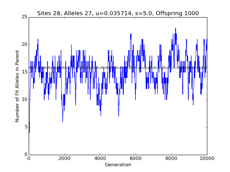
If you get an error message instead, and you’re not interested in Python programming, then give up. There are two main sources of problems. With an outdated version of the Numeric Python (numpy) module, you might see an error message ending with
AttributeError: 'module' object has no attribute 'choice'
or with
ValueError: n <= 0
Another possibility is that your Python is not configured to do graphics. I cannot help you with either problem. But, if you’re willing to Google for instructions, you can fix them. What I hope is that you’ll see a graphical display pop open, looking something like this.
If the display does not appear, check to see if it’s hidden behind other windows. No joy? Then there’s one last thing to try. Enter
$ python -i evolve.py
The -i stands for interactive, which is to say, you’re about to land back where non-programmers do not belong. But you’ve seen already what is most import to know — how to make the blasted thing quit(). Then again, it wouldn’t hurt simply to double-click the icon for the file evolve.py. If you’ve gotten this far, don’t give up. You can Google for instructions on how to configure the Python graphics backend. It might help to add the name of your operating system to the search term. If you learn something that stands to help other folks, please take a moment to post a comment here.

Your squiggly line will squiggle differently than mine, because there's randomness (or unpredictability that passes for randomness) involved. The solid line is the average value of the plotted quantity over the last 5000 generations. The dotted line is the prediction of the Wright-Fisher model, which does not apply strictly to the program. Much of the discrepancy is due, probably, to the shortness of the run. If you had not reduced N_GENERATIONS by a factor of 10, the solid line would have indicated the average of observations for 95 thousand generations, and probably would have been closer to the dotted line. The more generations in the run, the less variable the mean value of the observations (which determines the placement of the solid line).

Now, the point of all of this is to see how changing the parameters changes the behavior of the evolutionary process. You can learn quite a bit by repeatedly (1) editing the values of the inconstant constants (at the top of the file, with all-caps names), (2) saving the change, and (3) submitting the revised file to Python. And why do you have to do it this way? Because I have not learned how to do graphical user interfaces in Python. It doesn’t seem to be a priority at the moment. Then again, if I were any good at prioritizing, you wouldn’t have gotten this much out of me.

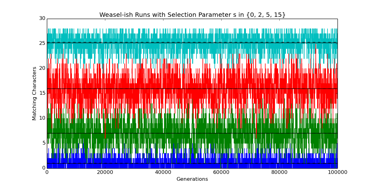
import numpy as np
import numpy.random as rand
import matplotlib.pyplot as plt

# Implement a model that is somewhat like Wright-Fisher, with Dawkins's Weasel
# as a special case.
# See Felsenstein (2016), "Wright, Fisher, and the Weasel," The Skeptical
# Zone, http://theskepticalzone.com/wp/wright-fisher-and-the-weasel/.
#
# Copyright Tom English, 2016.
# Permission for personal use granted. You may not redistribute this code,
# irrespective of whether you have modified or augmented it.


# The following are default values of model parameters.
# You can use a text editor to change the values between runs of the program.
# The all-caps notation tells programmers to change the values ONLY by editing.
#
N_SITES=28               # "Sentence length" (at least 1)
N_ALLELES=27             # "Alphabet size" (at least 2)
MUTATE_RATE=1.0/N_SITES  # Denoted u by Felsenstein (0.0 < u < 1.0)
N_OFFSPRING=1000         # Number of offspring per generation (at least 1)
SELECTION=5.0            # Denoted s by Felsenstein
N_GENERATIONS=100000     # Number of generations
EQUILIBRIUM_BEGIN=5000   # Evolution assumed stable after this many generations

assert(N_SITES >= 1)
assert(N_ALLELES >= 2)
assert(MUTATE_RATE > 0.0 and MUTATE_RATE < 1.0)
assert(N_OFFSPRING >= 1)


class Evolve(object):
    """
    Model somewhat like Wright-Fisher, with Dawkins's Weasel as a special case.
    """
    def __init__(self, n_sites=int(N_SITES), n_alleles=int(N_ALLELES), 
                       n_offspring=int(N_OFFSPRING), mutate_rate=MUTATE_RATE,
                       selection=float(SELECTION)):
        """
        Initialize evolutionary run.
        """
        self.n_sites = n_sites
        self.n_alleles = n_alleles
        self.n_offspring = n_offspring
        self.mutate_rate = mutate_rate
        self.selection = selection
        self.probability = np.empty(n_offspring, dtype=float)
        self.offspring = np.empty(n_offspring, dtype=int)
        self.n_fit = rand.binomial(N_SITES, 1.0 / n_alleles)
        self.history = [self.n_fit]

    def generation(self):
        """
        Extend evolutionary run by one generation.
 
        At each site, the allele is either fit or unfit.       
        The probability of selecting an offspring as parent of the next
        generation is proportional to its fitness `(1+selection)**n_fit`, 
        where `n_fit` is the number of fit alleles.
        """
        n = len(self.offspring)
        loss_rate = self.mutate_rate
        gain_rate = self.mutate_rate / (self.n_alleles - 1.0)
        self.offspring[:] = self.n_fit
        self.offspring += rand.binomial(self.n_sites - self.n_fit, gain_rate, n)
        self.offspring -= rand.binomial(self.n_fit, loss_rate, n)
        np.power(self.selection + 1.0, self.offspring, self.probability)
        self.probability /= np.sum(self.probability)
        self.n_fit = rand.choice(self.offspring, size=1, p=self.probability)
        self.history.append(self.n_fit)

    def extend(self, n_generations=N_GENERATIONS):
        """
        Extend evolutionary run by `n_generations` generations.
        """
        for _ in xrange(n_generations):
            self.generation()

    def get_history(self, begin=0, end=None):
        """
        Return list of nums. of fit alleles in parents for range of generations.
        """
        return self.history[begin:end]

    def report(self, begin=EQUILIBRIUM_BEGIN):
        """
        Report on some quantities addressed by Felsenstein (2016).
        """
        u = self.mutate_rate
        s = self.selection
        q = u / (1 + s * (1 - u))
        p = u * (1 + s) / (self.n_alleles - 1 + u * s)
        h = self.history[begin:]
        print '*'*72
        print 'Number of sites L               :', N_SITES
        print 'Number of possible alleles A    :', self.n_alleles
        print 'Number of offspring             :', len(self.offspring)
        print 'Mutation rate u                 :', u
        print 'Selection parameter s           :', s
        print 'p = u * (1 + s) / (A-1 + u * s) :', p
        print 'q = u / (1 + s * (1 - u))       :', q
        print 'Assume equilibrium at generation:', begin
        print 'W-F probability of fit allele at site p/(p+q)  :', p/(p+q)
        print 'Expected num. of fit alleles in parent Lp/(p+q):', N_SITES*p/(p+q)
        print 'Mean observed num. of fit alleles in parent    :', np.mean(h)
        print 'Std. dev. of observed numbers of fit alleles   :', np.std(h)
        print '*'*72
        plt.plot(self.history)
        m = np.mean(h)
        plt.plot((0, len(self.history)-1), (m, m), 'k-')
        m = N_SITES * p/(p+q)
        plt.plot((0, len(self.history)-1), (m, m), 'k--')
        plt.ylabel('Number of Fit Alleles in Parent')
        plt.xlabel('Generation')
        plt.title('Sites {0}, Alleles {1}, u={2:.6f}, s={3}, Offspring {4}'. \
                  format(self.n_sites,
                         self.n_alleles,
                         self.mutate_rate,
                         self.selection,
                         self.n_offspring))
        plt.show()


def example():
    """
    Plot numbers of fit alleles for runs varying in just one parameter.
    """
    plt.figure()
    n_generations = 100000      # Override the default N_GENERATIONS here
    equilibrium_begin = 5000    # Override the default EQUILIBRIUM_BEGIN here
    results = []
    for s in [0, 2, 5, 15]:     # Put other numbers in this list...
        e = Evolve(selection=s) # ... change `selection` to another parameter
        e.extend(n_generations)
        print 'Selection parameter s:', s
        e.report(begin=equilibrium_begin)
        results.append(e)
    plt.title('Weasel-ish Runs with Selection Parameter s in {0, 2, 5, 15}')
    plt.show()
    return results    


# Run with default parameter settings
plt.figure()
e=Evolve()
e.extend()
e.report()
plt.show()

# To run my example, intended primarily for programmers:
# results=example()

# Use plt.close('all') to close plots when interacting with Python.

Saturday, February 27, 2016

Felsenstein: Wright, Fisher, and the Weasel

Joe Felsenstein has posted a fine explanation of how Richard Dawkins’s monkey/Shakespeare model of cumulative selection, better known as the Weasel program, relates to the classic Wright-Fisher model in population genetics. The relation is approximate, because a finite set of offspring is sampled in the monkey/Shakespeare model, while an infinite set of offspring is sampled in the Wright-Fisher model. Joe raised the question of just how well certain results derived for a special case of Wright-Fisher apply to a Weasel-ish evolutionary process. And it happens that I had on hand some code that was easily adapted to address the question. I’m sharing it here, without explanation, and inviting readers to join the discussion at The Skeptical Zone.

A nice illustration of how nice Numeric Python array processing is…

… not that I’m going to explain it.

import numpy as np
import numpy.random as rand
import matplotlib.pyplot as plt


LENGTH=28
ALPHABET_SIZE=27
N_OFFSPRING=100


class Evolve(object):
    """
    Model somewhat like Wright-Fisher, with Dawkins's Weasel as a special case.

    See Felsenstein (2016), "Wright, Fisher, and the Weasel," The Skeptical
    Zone, http://theskepticalzone.com/wp/wright-fisher-and-the-weasel/.
    """
    def __init__(self, alphabet_size=ALPHABET_SIZE, n_offspring=N_OFFSPRING,
                 mutate_rate=1.0/LENGTH, selection=0.0):
        """
        Initialize evolutionary run.
        """
        self.alphabet_size = alphabet_size
        self.mutate_rate = mutate_rate
        self.selection = float(selection)
        self.probability = np.empty(n_offspring, dtype=float)
        self.offspring = np.empty(n_offspring, dtype=int)
        self.n_match = rand.binomial(LENGTH, 1.0 / alphabet_size)
        self.history = [self.n_match]

    def generation(self):
        """
        Extend evolutionary run by one generation.
        
        Probability of selecting an offspring is proportional to its fitness 
        `(1+selection)**n_match`, where `n_match` is the number of characters
        matching the target.
        """
        n = len(self.offspring)
        loss_rate = self.mutate_rate
        gain_rate = self.mutate_rate / (self.alphabet_size - 1.0)
        self.offspring[:] = self.n_match
        self.offspring += rand.binomial(LENGTH - self.n_match, gain_rate, n)
        self.offspring -= rand.binomial(self.n_match, loss_rate, n)
        np.power(self.selection + 1.0, self.offspring, self.probability)
        self.probability /= np.sum(self.probability)
        self.n_match = rand.choice(self.offspring, size=1, p=self.probability)
        self.history.append(self.n_match)

    def extend(self, n_generations=10000):
        """
        Extend evolutionary run by `n_generations` generations.
        """
        for _ in xrange(n_generations):
            self.generation()
            
    def get_history(self, begin=0, end=None):
        """
        Return list of numbers of matching sites for specified generations.
        """
        return self.history[begin:end]

    def report(self, begin=1000):
        """
        Report on some quantities addressed by Felsenstein (2016).
        """
        u = self.mutate_rate
        s = self.selection
        q = u / (1 + s * (1 - u))
        p = u * (1 + s) / (self.alphabet_size - 1 + u * s)
        h = self.history[begin:]
        print '*'*72
        print 'Sentence length L               :', LENGTH
        print 'Alphabet size A                 :', self.alphabet_size
        print 'Number of offspring             :', len(self.offspring)
        print 'Mutation rate u                 :', u
        print 'Selection parameter s           :', s
        print 'p = u * (1 + s) / (A-1 + u * s) :', p
        print 'q = u / (1 + s * (1 - u))       :', q
        print 'Assume equilibrium at generation:', begin
        print 'Theoretical prob. of match at site p/(p+q)   :', p/(p+q)
        print 'Expected number of matching sites Lp/(p+q)   :', LENGTH*p/(p+q)
        print 'Mean of observed numbers of matching sites   :', np.mean(h)
        print 'Std. dev. of observed nums. of matching sites:', np.std(h)
        print '*'*72
        plt.plot(self.history)
        m = np.mean(h)
        plt.plot((0, len(self.history)-1), (m, m), 'k-')
        m = LENGTH * p/(p+q)
        plt.plot((0, len(self.history)-1), (m, m), 'k--')


def example():
    """
    Plot numbers of matching sites for runs varying in just one parameter.
    """
    n_gens = 100000
    results = []
    for s in [0, 2, 5, 15]:
        e = Evolve(n_offspring=1000, selection=s, alphabet_size=27)
        e.extend(n_gens)
        print 'selection (s):', s
        e.report(begin=5000)
        results.append(e)
    plt.title('Weasel-ish Runs with Selection Parameter s in {0, 2, 5, 15}')
    plt.ylabel('Matching Characters')
    plt.xlabel('Generations')
    plt.show()
    return results

    
results=example()
# plt.close()

Clunky, but effective

Here’s the textual output corresponding to the four plots in the figure above, going from bottom to top (blue, green, red, cyan). The idea of this output is to make sure that I’m on the same page with other folks working on the problem.

selection (s): 0
************************************************************************
Sentence length L               : 28
Alphabet size A                 : 27
Number of offspring             : 1000
Mutation rate u                 : 0.0357142857143
Selection parameter s           : 0.0
p = u * (1 + s) / (A-1 + u * s) : 0.00137362637363
q = u / (1 + s * (1 - u))       : 0.0357142857143
Assume equilibrium at generation: 5000
Theoretical prob. of match at site p/(p+q)   : 0.037037037037
Expected number of matching sites Lp/(p+q)   : 1.03703703704
Mean of observed numbers of matching sites   : 1.02184187535
Std. dev. of observed nums. of matching sites: 0.97972454909
************************************************************************
selection (s): 2
************************************************************************
Sentence length L               : 28
Alphabet size A                 : 27
Number of offspring             : 1000
Mutation rate u                 : 0.0357142857143
Selection parameter s           : 2.0
p = u * (1 + s) / (A-1 + u * s) : 0.0041095890411
q = u / (1 + s * (1 - u))       : 0.0121951219512
Assume equilibrium at generation: 5000
Theoretical prob. of match at site p/(p+q)   : 0.252049180328
Expected number of matching sites Lp/(p+q)   : 7.05737704918
Mean of observed numbers of matching sites   : 7.03611540931
Std. dev. of observed nums. of matching sites: 2.26819646257
************************************************************************
selection (s): 5
************************************************************************
Sentence length L               : 28
Alphabet size A                 : 27
Number of offspring             : 1000
Mutation rate u                 : 0.0357142857143
Selection parameter s           : 5.0
p = u * (1 + s) / (A-1 + u * s) : 0.00818553888131
q = u / (1 + s * (1 - u))       : 0.00613496932515
Assume equilibrium at generation: 5000
Theoretical prob. of match at site p/(p+q)   : 0.571595558153
Expected number of matching sites Lp/(p+q)   : 16.0046756283
Mean of observed numbers of matching sites   : 15.9726634456
Std. dev. of observed nums. of matching sites: 2.5666185402
************************************************************************
selection (s): 15
************************************************************************
Sentence length L               : 28
Alphabet size A                 : 27
Number of offspring             : 1000
Mutation rate u                 : 0.0357142857143
Selection parameter s           : 15.0
p = u * (1 + s) / (A-1 + u * s) : 0.021534320323
q = u / (1 + s * (1 - u))       : 0.00230946882217
Assume equilibrium at generation: 5000
Theoretical prob. of match at site p/(p+q)   : 0.903141702516
Expected number of matching sites Lp/(p+q)   : 25.2879676704
Mean of observed numbers of matching sites   : 25.1902401027
Std. dev. of observed nums. of matching sites: 1.54315605955
************************************************************************

Wednesday, June 17, 2015

Responding to Dr. Ewert

I’ve added the following to A Question for Winston Ewert at The Skeptical Zone.


Dr. Ewert has responded nebulously at Uncommon Descent. I’d have worked with him to get his meaning straight. I’m not going to spend my time on deconstruction. However, I will take quick shots at some easy targets, mainly to show appreciation to [Elizabeth Liddle] for featuring this post as long as she has. Here, again, is what I put to Dr. Ewert:

Your search process decides when to stop and produce an outcome in the search space. A model may do this, but biological evolution does not. How do you measure active information on the biological process itself? Do you not reify a model?
Dr. Ewert seemingly forgets that to measure active information on a biological process is to produce a specific quantity, e.g., 109 bits.
One approach is to take the search space not to be the individual organisms, but rather the entire population of organisms currently alive on earth. Or one could go further, and take it to be the history of organisms during the whole of biological evolution. One could also take it to be possible spacetime histories. The target can then be taken to be spacetimes, histories, or populations that contain an individual organism type such as birds.
These search spaces roll off the tongue. But no one knows, or ever will know, what they actually contain. Even if we did know, no one would know the probabilities required for calculation of the active information for a given target. And even if we did know the probability of a given target for a given search, we would not be able to justify designating a particular probability distribution on the search space as the natural baseline. By the way, Dr. Ewert should not be alluding to infinite sets, as his current model of search applies only to finite sets.
Another possibility is to model evolution as a process which halts upon finding the target, but distinguish between the active information derived from the evolutionary process itself and the active information contributed by the stopping behavior. The stopping behavior cannot induce birds to show up in the first place, it can only select them as the output of the search when they arrive. By looking at the number of opportunities for birds to arise, we can determine how much active information was added by the stopping process. It was shown in Conservation of Information in Search: Measuring the Cost of Success that the active information available from such a process is only the logarithm of the number of queries. Any other active information must derive from the evolutionary search itself.
Dembski and Marks define search differently in the cited paper than Dembski, Ewert, and Marks do. The result that Dr. Ewert invokes does not apply to the active information of a search, as presently defined. With the current definition, we can specify a process that goes through elements of the finite search space, one by one, until it recognizes an element of the target. Then the active information of the process is due almost entirely to recognition of the target by the stopping process. I hope this gives you some idea of what’s wrong with Ewert’s claim. Perhaps one of the cognoscenti will supply more of the details in a comment.
Both approaches effectively end up adjusting for the number of trials. Getting a royal flush is improbable, but if you play five million hands of poker it is no longer surprising. Similarly, obtaining a bird is rendered much more probable given the number of chances for it happen in the history of universe. It is a very important point to keep in mind that we cannot simply look at the probability of the individual events but also the number of trials.
Dr. Ewert errs, and has brought to the fore a major weakness of the current definition of search. Here the search space is the set of all five-card poker hands, and the target is the subset containing the royal-flush hands. A search that halts after one step and yields a royal flush with probability 1/2 has exactly the same active information as a search that yields a royal flush with probability 1/2 after five million or fewer steps. In short, a very important point to keep in mind is that the number of trials actually does not enter into the calculation of active information.
For birds to have been produced by an evolutionary process, the universe must have been biased towards producing birds.
Must the universe have been biased against producing flying insects that walk on all fours? (This is not a cheap dig at religion, but instead a substantive response to Robert Saying the Bible is not a book about science is like saying a cookbook is not a book about chemistry Marks. I had forgotten Leviticus 11:20 until I Googled for scientific discussion of why there are no four-legged insects.)

Wednesday, June 3, 2015

At least a hint, Dr. Ewert?

Posted in The Skeptical Zone.


I repeat my invitation to Dr. Winston Ewert to join us here for discussion of several questions I raised. It helps immensely to display mathematical formulas, rather than talk about them vaguely. However, he has replied at Uncommon Descent, where that is impossible. I’m genuinely astonished to see:

Thursday, May 14, 2015

A better reason for Dr Ewert to enter The Skeptical Zone

As I explained in my last post, Winston Ewert has solicited questions on his research with William Dembski and Robert Marks, and I have raised several at The Skeptical Zone. I avoided upstaging DiEb, who followed Ewert’s procedure, and submitted questions through a Google Moderator page. As you can see from the following note I left at DiEblog, an immoderate moderator at Uncommon Descent has haplessly given Ewert a better reason to answer at The Skeptical Zone than I have.


I hope you don’t mind my observation that your post relates to one of three questions you posed at Ask Dr Ewert (link expires June 30, 2015). Ewert, who collaborates with Dembski and Marks, evidently intends to answer selected questions at Uncommon Descent. You’ve been banned there since raising the questions, have you not? Correlation does not imply causation. But if you cannot comment on his answers to your questions, then he will in fact have ensconced them in a sham forum.

Tuesday, May 12, 2015

At The Skeptical Zone: A question for Winston Ewert

I’ve invited Winston Ewert to join a technical discussion at The Skeptical Zone. I do solemnly vow to keep it perfectly civil. It would be better to comment there than here. But suit yourself.


I actually have three technical questions for Winston, but plan on one post apiece. He should respond first to questions he receives through Google Moderator, including those from DiEb, who has added a relevant post to his blog. Hopefully he will join us here when he’s done with that.

Let’s be clear from the outset that off-topic remarks go straight to Guano. (If you attack Winston personally while I am trying to draw him into a discussion of theory, then I will take it personally.) You shouldn’t make claims unless you have read, and believe that you mostly understand, the material in all three sources in note 3, apart from the proofs of theorems. Genuine requests for explanation are, of course, welcome. They’re especially welcome if you’ve made a genuine effort to get what you can from the sources.

The overall thrust of my questions should be clear enough to Winston, though it won’t be to most readers. I’m definitely not laying a trap for him. The first two questions have answers that are provably right or wrong. The third is more a matter of scientific modeling than of math. I’m starting with it because TSZ isn’t yet configured to handle embedded LaTeX (mathematical expressions).

Questions

1. What is the formal relationship between active information and specified complexity?

2. What is the formal relationship between active information and average active information per query? Does the conservation-of-information theorem apply to the latter?

3. Your search process decides when to stop and produce an outcome in the search space. A model may do this, but biological evolution does not. How do you measure active information on the biological process itself? Do you not reify a model?

Notes

1. There’s an answer that covers both Dembski's 2005 version (the probabilistic complexity minus the descriptive complexity of the target) and the algorithmic version of specified complexity. For the latter, it’s apparently necessary to restrict the target (no longer called a target) to a single-element set.

2. The conservation-of-information theorem applies to active information. Winston and his colleagues have measured only average active information per query (several closely related forms, actually), which seems unrelated to active information, in their analyses of computational evolution and metabiology. Yet they refer to conservation of information in exposition of those analyses.

3. The search process of Dembski, Ewert, and Marks terminates, and generates an outcome. The terminator and the discrim­inator of the search in fact contribute to its active information — bias, relative to a baseline distribution on outcomes, in favor of a target event. However, biological evolu­tion has not come to a grinding halt, and has not announced, for instance, Here it is — birds! It seems that Winston, in his ENV response to a Panda’s Thumb post by Joe Felsenstein and me, tacitly assumes that a biologist has provided a model that he can analyze as a search, and imputes to nature itself the bias that he would measure on the model of nature. If so, then he erroneously treats an abstraction as though it were something real. Famously, The map is not the territory. Perhaps Winston can provide a good argument that he hasn’t lapsed into reification.

Sunday, March 29, 2015

Deobfuscating a theorem of Ewert, Marks, and Dembski

Back in July, I found that I couldn’t make heads or tails of the theorem in a paper by Winston Ewert, Robert J. Marks II, and William A. Dembski, On the Improbability of Algorithmic Specified Complexity. As I explained,

The formalism and the argument are atrocious. I eventually decided that it would be easier to reformulate what I thought the authors were trying to say, and to see if I could generate my own proof, than to penetrate the slop. It took me about 20 minutes, working directly in LaTeX.
I posted a much improved proof, but realized the next day that I’d missed something very simple. With all due haste, here is that something. The theorem is best understood as a corollary of an underwhelming result in probability.

The simple

Suppose that $\mu$ and $\nu$ are probability measures on a countable sample space $\Omega$, and that $c$ is a positive real number. What is the probability that $\nu(x) \geq c \cdot \mu(x)$? That’s a silly question. We have two probabilities of the event \[ E = \{x \in \Omega \mid \nu(x) \geq c \cdot \mu(x) \}. \] It’s easy to see that $\nu(E) \geq c \cdot \mu(E)$ when $\nu(x) \geq c \cdot \mu(x)$ for all $x$ in $E$. The corresponding upper bound on $\mu(E)$ can be loosened, i.e., \begin{equation*} \mu(E) \leq \frac{\nu(E)}{c} \leq \frac{1}{c}. \end{equation*} Ewert et al. derive $\mu(E) \leq c^{-1}$ obscurely. [Added 30/12/2018: George Montañez has referred to this post in his BIO-Complexity article “A Unified Model of Complex Specified Information.” I should make explicit something that is implied by the identification, below, of $\nu$ with an algorithmic probability measure: there is no requirement that the probabilities of atomic outcomes sum to unity, i.e., that $\mu(\Omega) = 1$ and $\nu(\Omega) = 1.$ The loosening of the upper bound on $\mu(E)$ assumes that $\nu(\mathcal{E}) \leq 1$ holds for all events $\mathcal{E} \subseteq \Omega.$]

The information-ish

To make the definition of $E$ information-ish, assume that $\mu(x) > 0$ for all $x$ in $\Omega$, and rewrite \begin{align} \nu(x) &\geq c \cdot \mu(x) \nonumber \\ \nu(x) / \mu(x) &\geq c \nonumber \\ \log_2 \nu(x) - \log_2 \mu(x) &\geq \alpha, \end{align} where $\alpha = \log_2 c$. This lays the groundwork for über-silliness: The probability of $\alpha$ or more bits of some special kind of information is at most $2^{-\alpha}$. This means only that $\mu(E) \leq c^{-1} = 2^{-\alpha}.$

The ugly

Now suppose that $\Omega$ is the set of binary strings $\{0, 1\}^*$. Let $y$ be in $\Omega$, and define an algorithmic probability measure $\nu(x) = 2^{-K(x|y)}$ for all $x$ in $\Omega$. (I explained conditional Kolmogorov complexity $K(x|y)$ in my previous post.) Rewriting the left-hand side of Equation (1), we obtain \begin{align*} \log_2 2^{-K(x|y)} - \log_2 \mu(x) &= -\!\log_2 \mu(x) - K(x|y) \\ &= ASC(x, \mu, y), \end{align*} the algorithmic specified complexity of $x$. Ewert et al. express an über-silly question, along with an answer, as \[ \Pr[ASC(x, \mu, y) \geq \alpha] \leq 2^{-\alpha}. \] This is ill-defined, because $ASC(x, \mu, y)$ is not a random quantity. But we can see what they should have said. The set of all $x$ such that $ASC(x, \mu, y) \geq \alpha$ is the event $E$, and $2^{-\alpha} = c^{-1}$ is a loose upper bound on $\mu(E)$.

Tuesday, March 10, 2015

Tolstoy on the studious deceit of children by the church

Nothing captures my experience with the church better than does this passage from Leo Tolstoy’s The Kingdom of God is Within You (1894).

The chief and most pernicious work of the Church is that which is directed to the deception of children — these very children of whom Christ said: Woe to him that offendeth one of these little ones. From the very first awakening of the consciousness of the child they begin to deceive him, to instill into him with the utmost solemnity what they do not themselves believe in, and they continue to instill it into him till the deception has by habit grown into the child's nature. They studiously deceive the child on the most important subject in life, and when the deception has so grown into his life that it would be difficult to uproot it, then they reveal to him the whole world of science and reality, which cannot by any means be reconciled with the beliefs that have been instilled into him, leaving it to him to find his way as best he can out of these contradictions.

If one set oneself the task of trying to confuse a man so that he could not think clearly nor free himself from the perplexity of two opposing theories of life which had been instilled into him from childhood, one could not invent any means more effectual than the treatment of every young man educated in our so-called Christian society.

(I provide context here.) It’s not exactly surprising that people who refer to indoctrination as Christian education should regard education as indoctrination when it happens to conflict with their beliefs.

Sunday, September 28, 2014

Would E.T. notice an icon of ID creationism?

Robert J. Marks II in his article on IDC in the conservative political outlet Human Events:

Yet we all agree that a picture of Mount Rushmore with the busts of four US Presidents contains more information than a picture of Mount Fuji.
As Jeff Shallit indicates, no, we really don’t. He has formal measures of information in mind, as I usually do. But I’ve posted a lot of formal stuff lately, and I’m going to do something more intuitive. [What you see here is an abortive attempt at late-night writing from over a month ago. Now that Jeff has posted a note he sent to Marks, I'm going to let it go as is. The pictures are fun.]

Is there some special kind of information in an image of Mount Rushmore that would grab the attention of an extraterrestrial flying by? A bright patch is certainly noticeable, but I don’t think that qualifies as a special kind of information, or as much information of any kind. And as lichen grows on the sculpture, it darkens. (This video has before-and-after shots at 4:50.) If you want to know what really wows E.T., click on the image below.


Photo by Volkan Yuksel (cropped).

There may well be a “look here, look here” icon long after the faces have crumbled.

Am I playing a dirty trick? No, by showing you the big picture, I’m allowing you to see that the form of the sculpture does not stand out from the rest of the mountain. It could not have been otherwise. A sculptor subtracts from what is already present to arrive at the result. Even when the medium is marble, there are sometimes features that drive the composition (see the quotes of Michelangelo and Henry Moore in a past post). Gutzon Borglum could not simply imagine the form of the monument, and then pick a mountain arbitrarily. He had to study available mountain form-ations, and imagine what he could produce by removing modest amounts of material.

Am I trying to diminish the work of Borglum? Certainly not. For someone to envision a monument in the side of a mountain is amazing. My point is that much of the form-ation of the sculpture was already done. The in-form-ation by the sculptor was relatively fine detail, for the most part, and that is why the gross features do not stand out from the surrounding stone.

Of course, the ID creationists make E.T. get up close and personal. The point has been made a gazillion times that an extraterrestrial may be so unlike a person that faces mean nothing to it. What objectively stands out in a shot that is tighter, but not as tight as the IDCists want it to be, is the relatively flat surface surrounding the heads. The pile of rubble beneath the carving also draws attention to it. How ironic.

The IDCists always frame what they say contains some sort of special information, without accounting for how that happens. Put simply, why does E.T. zoom in on a relatively small part of Mount Rushmore, if it doesn’t stand out? To come at this another way, Marks expects us to compare the typical image of Mount Fuji, far in the distance, to the typical image of Mount Rushmore, which is a small part containing the sculpture. That is what prompted me to go looking for shots from different perspectives and different distances. [… “If you want any more, you can sing it yourself.”]


"Mountfujijapan" by Swollib


Special Added Bonus Feature: Creationist Persecution Fantasy